A Physics Informed Neural Network for 1D Heat Transfer
Physics-Informed Neural Networks (PINNs) are a promising way to blend deep learning with physical laws. This typically allows us to solve differential equations without needing traditional numerical discretization methods. In this post, I look at a simple example to show how PINN can be used to solve an engineering problem, one-dimensional heat transfer.
Although the one-dimensional heat equation is a trivial problem when compared with more complex engineering scenarios, it can serve as an excellent starting point to understand the mechanics behind PINNs. These ideas can be extended to solve multidimensional and highly nonlinear engineering problems.
Before we look at implementing PINN to solve 1D heat transfer problem, I first look at how we can calculate the numerical derivatives using auto-differentiation in TensorFlow.
Auto-Differentiation in TensorFlow
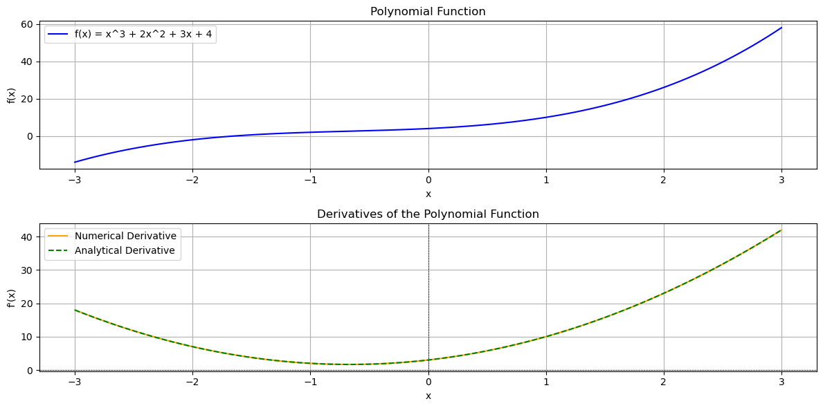
One of the key features of PINNs is the use of automatic differentiation. TensorFlow’s “GradientTape” records operations on tensors to compute derivatives. Consider the simple polynomial function:
\[f(x) = x^3 + 2x^2 + 3x + 4\]Its analytical derivative is:
\[f'(x) = 3x^2 + 4x + 3\]Below is a code snippet that shows how to get the derivative using TensorFlow:
import tensorflow as tf

# This is the original function
def polynomial_function(x):
    return x**3 + 2*x**2 + 3*x + 4

# Here, we create a TensorFlow variable named x_tf with an initial value of 2.0. This represents the input value for which we want to compute the derivative.
x_tf = tf.Variable(2.0)

# This is how we keep a record of operating on tensors that involve differentiable computations. TensorFlow will later use this recorded information to compute gradients.
with tf.GradientTape() as tape:
    # This line computes the value of the desired function (in this case, a polynomial) using the variable x_tf as input.
    y_tf = polynomial_function(x_tf)

# Now that we have the derivative recorded within "tape", we can compute the derivative of y_tf with respect to x_tf.
numerical_derivative = tape.gradient(y_tf, x_tf)
print("Numerical derivative at x=2.0:", numerical_derivative.numpy())
In this snippet, GradientTape “watches” the variable x_tf. Every operation on x_tf is recorded so that TensorFlow can automatically compute the derivative. You can see the complete code for comparing the analytical derivative and the one calculated using this approach at this address. The output for this function is as follows:
This same mechanism isused when computing derivatives with respect to spatial and temporal variables in the PINN example later.
Now, with this in mind, let’s look at the example of one-dimensional heat transfer problem with given boundary and initial conditions.
PINNs for 1D Heat Transfer
The 1D heat equation is given by:
\(u_t = \alpha \ u_{xx}\)
where:
- \(u(x, t)\) is the temperature distribution.
- \(u_t\) is the time derivative,
- \(u_{xx}\) is the second spatial derivative, and
- \(\alpha\) is the thermal diffusivity.
In our PINN approach, the neural network learns a mapping from (x, t) to u(x, t) such that the network output satisfies the heat equation, initial condition, and boundary conditions.
Neural Network Structure
The network is designed to take two inputs (x and t) and produces one output (u), usually through a series of fully connected layers. A common architecture might be:
- Input layer of size 2 for (x, t).
- Two or more hidden layers with multiple neurons each and an activation function.
- One output neuron representing the predicted temperature.
Below is a representative snippet for defining the neural network:
import tensorflow as tf

model = tf.keras.Sequential([
    tf.keras.layers.Input(shape=(2,)),               # (x, t) input
    tf.keras.layers.Dense(50, activation='tanh'),    # first hidden layer
    tf.keras.layers.Dense(50, activation='tanh'),    # second hidden layer
    tf.keras.layers.Dense(1)                         # output layer: u(x, t)
])
model.build((None, 2))  # Initializing weights by building the model
Embedding the Physics
Instead of training solely on data, a PINN embeds the differential equation into the loss function. We compute the derivatives u_t and u_xx using TensorFlow’s GradientTape and define a residual that must be minimized:
def loss_function(X, t, alpha):
    # Here, we combine inputs for the forward pass
    with tf.GradientTape(persistent=True) as tape:
        tape.watch(X)
        tape.watch(t)
        U = model(tf.concat([X, t], axis=1))  # predicting temperature

        # Then, we compute first derivatives with respect to x and t
        U_t = tape.gradient(U, t)
        U_x = tape.gradient(U, X)
        # and second derivative with respect to x
        U_xx = tape.gradient(U_x, X)

    # We then define the residual as u_t - alpha*u_xx, which should be close to zero based on the governing equation
    residual = U_t - alpha * U_xx

    del tape
    return tf.reduce_mean(tf.square(residual))
Notice that we are only computing the residual from the heat equation. Next, we enforce the boundary and initial conditions.
Incorporating Boundary and Initial Conditions
In the 1D heat problem, the boundary conditions might be prescribed, for example, here we consider \(u(0, t) = 0\) and \(u(L, t) = 0\), which are Dirichlet conditions for the rod’s ends. Similarly, the initial condition can also be defined as \(u(x, 0) = sin(\pi x)\), which is a common test case with a known analytical solution.
I am now going to add their contributions to the overall loss function as follows:
def boundary_conditions_loss(L, t):
    u_left = model(tf.concat([tf.zeros_like(t), t], axis=1))  # u(0,t)=0
    u_right = model(tf.concat([L * tf.ones_like(t), t], axis=1))  # u(L,t)=0
    return tf.reduce_mean(tf.square(u_left)) + tf.reduce_mean(tf.square(u_right))

def initial_conditions_loss(N_x, L):
    x_initial = tf.convert_to_tensor(np.linspace(0, L, N_x)[:, None], dtype=tf.float32)
    t_initial = tf.zeros_like(x_initial, dtype=tf.float32)
    u_initial_pred = model(tf.concat([x_initial, t_initial], axis=1))
    u_initial_true = tf.sin(np.pi * x_initial)
    return tf.reduce_mean(tf.square(u_initial_pred - u_initial_true))
Complete Loss Function
The complete loss would sum the PDE residual loss, the boundary condition loss, and the initial condition loss as follows:
def loss_function(X, t):
    with tf.GradientTape(persistent=True) as tape:
        tape.watch(X)
        tape.watch(t)
        U = model(tf.concat([X, t], axis=1))
        U_t = tape.gradient(U, t)
        U_x = tape.gradient(U, X)
        U_xx = tape.gradient(U_x, X)

    residual = U_t - alpha * U_xx
    bc_loss = boundary_conditions_loss(L, t)
    ic_loss = initial_conditions_loss(N_x, L)

    # This is our complete loss function, including initial condition, boundary condition, and residual loss (representing the physics of the problem)
    total_loss = tf.reduce_mean(tf.square(residual)) + bc_loss + ic_loss

    del tape

    return total_loss
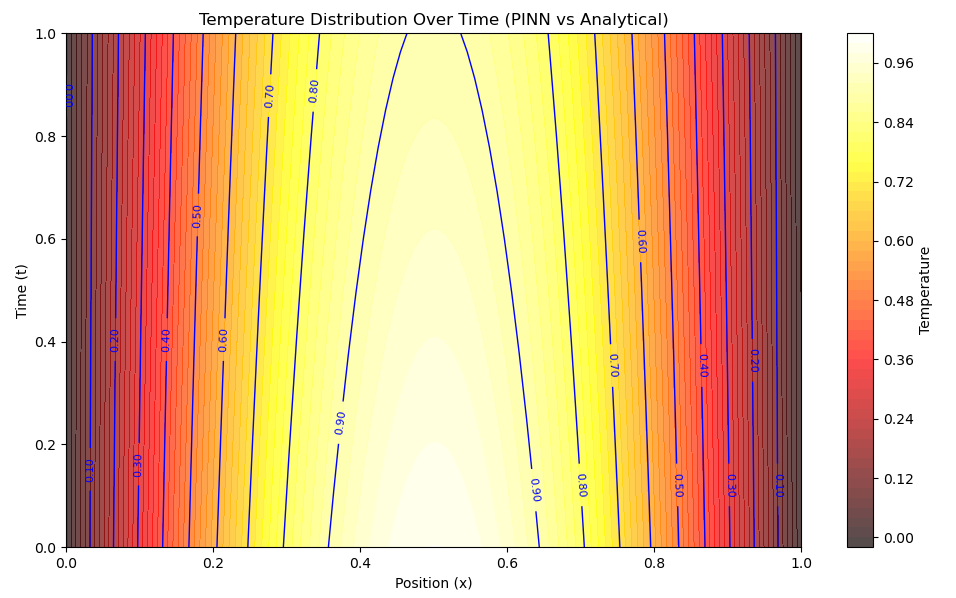
Training adjusts the network’s weights to minimize the combined loss. This optimization process produces a model that simulates heat transfer accurately compared to the analytical solution.
Training the PINN
The network is optimized using an algorithm like Adam, which makes small adjustments to the weights based on the computed loss values. A simplified training loop might look like this:
optimizer = tf.keras.optimizers.Adam(learning_rate=0.001)
loss_history = []
for epoch in range(10000):
    with tf.GradientTape() as tape:
        loss = loss_function(X_flat_tf, t_flat_tf)

    grads = tape.gradient(loss, model.trainable_variables)

    optimizer.apply_gradients(zip(grads, model.trainable_variables))
    loss_history.append(loss.numpy())

    if epoch % 1000 == 0:
        logging.info(f'Epoch {epoch}, Loss: {loss.numpy()}')
The loop above iteratively improves the neural network so that the output function \(u(x, t)\) satisfies the heat equation as well as the imposed initial and boundary conditions. Here is a comparison between the analytical solution and the output from the trained PINN.
For a full implementation of the complete PINN for 1D heat transfer, check out this link.
Why This Example Matters
This 1D heat transfer example is trivial in the sense that the analytical solution is known. However, the same principles apply to far more complex problems in engineering mechanics, including:
- Multidimensional heat transfer in irregular geometries.
- Fluid-structure interactions where the governing equations are highly nonlinear.
- Coupled phenomena in material science or biomechanics.
For such problems, traditional numerical methods (e.g., finite element or finite difference) might struggle with mesh generation, handling complex boundaries, and high-dimensional parameter spaces. PINNs, in contrast, handle these issues by embedding the physics directly into the neural network’s loss function, offering a mesh-free and flexible computational framework.
Enjoy Reading This Article?
Here are some more articles you might like to read next: